Step-by-Step Guide to the Gaussian Basis Regression

In this post, I will go over Gaussian Basis Regression, a technique used in machine learning to model complex relationships between features and labels. I include both the mathematical background and the practical implementation using Python.

What’s Gaussian Basis Regression?

Gaussian Basis Regression is a type of regression analysis where feature vectors are transformed using Gaussian functions.

What this means is that if we have a hypothesis function of the form:

Instead of using input featuresdirectly, we use feature map:

Thus our hypothesis function becomes:

We can use different types of basis function, but in this case, we will use Gaussian functions. Let’s choose Gaussian function $\phi_{\sigma,\mu}(x) = \exp\!\Bigl(-\tfrac{1}{2\,\sigma^2}\,\bigl(x - \mu\bigr)^2\Bigr)$ as the basis function.

Thus our design matrix will be:

Why Gaussian Basis Regression?

Why should we use Gaussian Basis Regression over Polynomial Regression or other types of regression?

The main reason is that gaussian basis regression is localized. This means that each basis function is only active in a small region of the input space. This is useful when we have data that is not linear, but we don’t know where the non-linearity is.

For example, let’s give an example of non-linear data:

Consider temperature data from a city. The temperature at the morning is low, then it sharply increases in the afternoon. At the middle of the day the temperature can be high, but in the evening it decreases again.

This type of change is not linear, but it is localized, e.g., we can estimate the temperature by Gaussian function that are centered at the morning, afternoon, and evening. Each of these Gaussian functions will be active in a small region of the input space, and will help us to estimate the temperature in that given region only!

Three Hyperparameters

When setting up Gaussian function, we defined three hyperparameters that we need to choose:

1. Number of Basis Functions (M)

Number of Basis Functions (M) is term that tells us how many Gaussian functions we will use in our model. Let’s give an example:

Let’s choose M=3, thus the design matrix becomes:

for j=1,2,3.

2. Centers (μ)

We first chose how many functions we will use, and now we need to choose where to place these functions. Centers (μ) is term that tells us where our Gaussian functions will be centered.

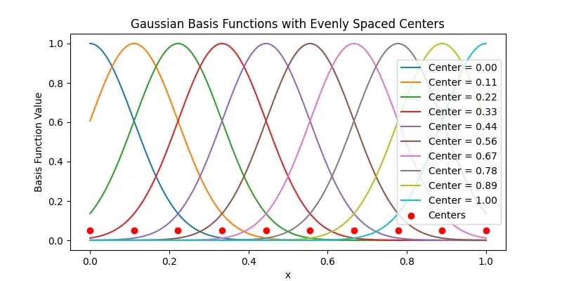
There are different ways to choose centers, simplest is evenly by the data range. We could also use k-means clustering or other methods to choose the centers.

Here’s image where I have plot Gaussian functions with centers chosen evenly by the data range.

3. Standard Deviation (σ)

Standard Deviation (σ) is term that tells us how wide our Gaussian functions will be. This can also be understood as how big area of the data our Gaussian function will cover, bigger the area, more data points will be covered by the function.

Common choice is to set σ to be equal to the distance between two adjacent centers.

Ordinare Least Squares

Now that we know what are the hyperparameters for our Gaussian function. We can finally start talking how to optimize our model.

Our predictions are in the form:

To learn the weights, we can define a loss function and minimize it. One common choice is the Sum of Squared Errors (SSE) loss function.

Let’s expand this into quadratic formula.

And to further simplify it, we know that

and

Thus our loss function becomes

From here we notice, that this actually is quadratic form!

Where $A=\Phi^{\top} \Phi$ , $b=-2y^{T}\Phi$ and $c=y^{T}y$

And because it’s in quadratic form, we can solve it by linear algebra if $A$ is invertible.

This is done by taking the gradient w.r.t w.

And by setting it to zero, we get

Finally we can calculate the optimal weights!

Python Implementation

Now that we know the math behind it, let’s implement it in Python!

First, as always, we need to get some data. I will generate some synthetic data. This time my data will be:

And here’s the code for it:

import numpy as np
import matplotlib.pyplot as plt

np.random.seed(42)
x = np.linspace(0, 1, 400)
noise = np.random.normal(0, 0.1, size=x.shape)
y = np.sin(2 * np.pi * x) + noise

After that we need to define the hyperparameters of the Gaussian function.

I will use 10 evenly spaced centers, which width is the same as the distance between the centers.

def gaussian_basis(x, centers, width):
    return np.exp(-(x[:, None] - centers)**2 / (2 * width**2))

M = 10
centers = np.linspace(0, 1, M)
sigma = (centers[1] - centers[0])
Phi = gaussian_basis(x, centers, sigma)

Now to get the weights, we just need to solve the normal equations by the formula that we saw before.

def solve_normal_equations(Phi, y):
    return np.linalg.inv(Phi.T @ Phi) @ Phi.T @ y

w = solve_normal_equations(Phi, y)

Notice how simple it is to solve the weights in this. However, this is good if the number of features or training examples is small. For large datasets, computing the inverse matrix can be computationally expensive and numerically unstable.

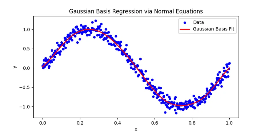
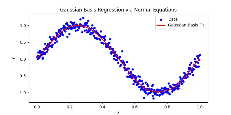
Finally, we can plot the results of the regression and see if it fits well.

x_plot = np.linspace(0, 1, 200)
Phi_plot = gaussian_basis(x_plot, centers, sigma)
y_plot = Phi_plot @ w

plt.figure(figsize=(8, 4))
plt.scatter(x, y, color="blue", label="Data", s=20)
plt.plot(x_plot, y_plot, color="red", label="Gaussian Basis Fit", linewidth=2)
plt.xlabel("x")
plt.ylabel("y")
plt.title("Gaussian Basis Regression via Normal Equations")
plt.legend()
plt.show()

As we can see, our simple model fits the data very well! Even though the data has some noice, the underlying model captures the trend of data.

Conclusion

In this post, we saw how to use Gaussian basis functions to fit a non-linear model to data. We also solved how to solve the weights using the normal equations.

For the full code, you can check out the GitHub repository.