Implementing Polynomial Regression from Scratch

In this post I will be implementing polynomial regression from scratch. This is a follow up post to my linear regression from scratch. post.

Polynomial Regression vs Linear Regression

Polnomial regression is an extension of the linear regression model. Instead of working with linear maps such as:

Polynomial maps are constructed by adding higher order terms to the linear map:

As in the linear regression, we can use squared error loss (MSE) to train the model. The goal is the same, get the weights that minimize the loss function.

Using Gradient Descent in Polynomial Regression

To minimize the loss function we can use gradient descent, as in the linear regression model. However, due to polynomial regression having higher order terms, we need to use a different approach to calculate the gradients.

Let’s calculate the gradient for n degree polynomial regression.

Our loss function is exactly the same as in linear regression:.

We first need partial derivates for each weight. Let’s calculate the partial derivate for w_j.

Let’s first define error variable $e^{i} = y^{i} - h(x^{i})$ From this, our loss function can be written as: $L(w) = (1/M)\sum_{i=1}^{m}(e^{i})^{2}$

Using the chain rule, we can calculate the partial derivate for $w_j$ as follows:

Since $e_{i} = y^{i} - h(x^{i})$ , we have: $\frac{\delta e_{i}}{\delta w_{j}} = -\frac{\delta h(x^{i})}{\delta w_{j}}$

But $h(x^{i}) = w_{0} + w_{1}x_{1}^{i} + w_{2}(x_{1}^{i})^{2} + ... + w_{n}(x_{1}^{i})^{n}$ , so: $\frac{\delta h(x^{i})}{\delta w_{j}} = (x_{i})^{j}$

Combining these results, we get:

Thus we can use this formula to update the weights in the gradient descent algorithm!

Code Implementation

Now let’s see how can we implement this in Python!

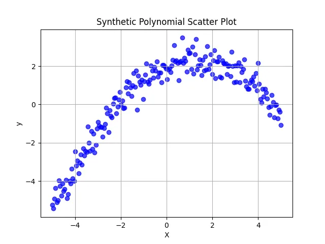
First we need some data, I chose to generate this data:

import numpy as np
import pandas as pd
import matplotlib.pyplot as plt

np.random.seed(43)
X = np.linspace(-5, 5, 200)
# True polynomial: y = 2 + 0.5 X - 0.2 X^2 + noise
y = 2 + 0.5*X - 0.2*X**2 + np.random.normal(scale=0.5, size=X.shape)

df_synthetic = pd.DataFrame({'X': X, 'y': y})

Here’s the plot of the data, we can see that it’s highly non-linear:

After that we prepare the data to be used in the model by splitting it into train and test sets and scaling it:

X_data = df_synthetic["X"].values
y_data = df_synthetic["y"].values

N = len(X_data) # Number of Data Points
train_ratio = 0.8 # Train-Test Split Ratio
train_size = int(N * train_ratio)

# Shuffle Data
indices = np.random.permutation(N)
train_idx, test_idx = indices[:train_size], indices[train_size:]

X_train, y_train = X_data[train_idx], y_data[train_idx]
X_test, y_test = X_data[test_idx], y_data[test_idx]

X_mean = X_train.mean()
X_std = X_train.std()

X_train_scaled = (X_train - X_mean) / X_std
X_test_scaled = (X_test - X_mean) / X_std

Then I define the model and the loss function that are needed to train the model. Notice these are very simple implementations, just polynomial function and mean squared error.

def model(X, theta):
    y_pred = 0
    for i in range(len(theta)):
        if i == 0:
            y_pred = theta[i]
        else:
            y_pred += theta[i] * X**i
    return y_pred

def loss(y_true, y_pred):
    return np.mean((y_true - y_pred)**2)

Finally we can train the model using gradient descent.

degrees = range(1, 6) # Polynomial Degree
fig, axs = plt.subplots(2, 3, figsize=(20, 8))
axs = axs.flatten()

for idx, deg in enumerate(degrees):
   theta = np.zeros(deg + 1)
   learning_rate = 1e-4
   n_iter = 50000

   for i in range(n_iter):
       predictions = model(X_train_scaled, theta)
       error = y_train - predictions  # (y - y_pred)

       gradients = np.zeros_like(theta)
       for j in range(len(theta)):
           gradients[j] = -2 * np.mean(error * (X_train_scaled ** j))

       
       theta -= learning_rate * gradients

The code simply goes over different degrees of polynomials and trains the model using gradient descent. Notice that the gradient is calculated for each parameter same way as in the math section above! Now error = e, and $\theta_{j} = w_{j}$

Finally, I evaluate the best model out of the different degrees and plot the results.

MSE_train = loss(y_train, model(X_train_scaled, theta))
MSE_test = loss(y_test, model(X_test_scaled, theta))
r2_score_train = r2_score(y_train, model(X_train_scaled, theta))
r2_score_test = r2_score(y_test, model(X_test_scaled, theta))

I get this kind of results:

Degree	Train Loss	Test Loss	Train R2 Score	Test R2 Score
1	2.21	3.16	0.47	0.44
2	0.27	0.21	0.94	0.96
3	0.29	0.23	0.93	0.96
4	0.33	0.29	0.92	0.95
5	0.33	0.28	0.92	0.95

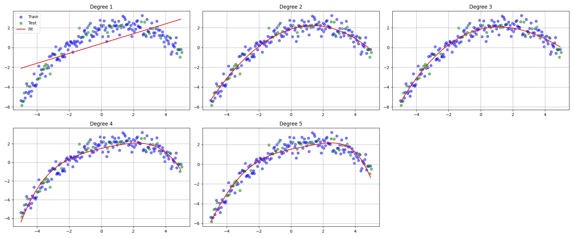
By looking at the results, we can see that the model with degree 2 is the best model, as it has the lowest test loss and the highest test R2 score.

Conclusion

In this project, I implemented polynomial regression from scratch using gradient descent. The math behind polynomial regression is very similar to linear regression, but with the addition of polynomial features.

Check out the full code on my GitHub repository.