Linear Regression from Scratch using Python

Linear regression is a simple machine learning model that predicts in linear hypothesis space. In this post, I’ll show how to create simple linear regression model by using Python and NumPy. I’ll give code samples and the math behind the model to help you understand how it works.

What is Linear Regression?

Linear regression is a simple machine learning model that predicts the label based on the linear hypothesis space. The simplest form of linear regression is a linear equation that models the relationship between the dependent variable y and the independent variable x as:

h(x) = w_{1}x + w_{0}

Where:

h(x) is the hypothesis mapping function
x is the feature
$w_{0}$ , $w_{1}$ are the weights

The goal of the linear regression is to find the best weights w_0, w_1 that minimize the error between the predicted value and the actual value. Thus we can choose our loss function as Mean Squared Error (MSE) which is defined as:

1 / m \sum_{i = 1}^{m}(y^{i} - h(x^{i}))^{2}

Where:

$m$ is the number of samples
$y^{i}$ is the actual value
$h(x^{i})$ is the predicted value

Now, our goal is to minimize the loss function by updating the weights. Thus the goal is to find:

\hat{\textbf{w}}= argmin (1 / m) \sum_{i = 1}^{m}(y^{i} - h(x^{i}))^{2}

Gradient Descent

We now know what we want to minimize, but how do we do it? One way to do this is by using the gradient descent algorithm. Gradient descent is an optimization algorithm that minimizes the loss function by iteratively updating the weights in the opposite direction of the gradient of the loss function.

So let’s calculate the gradient of the loss function with respect to the weights:

\nabla_{\textbf{w}} = \begin{bmatrix} \frac{\partial L}{\partial w_{0}} \\ \frac{\partial L}{\partial w_{1}} \end{bmatrix}

These partial derivates can be calculated as:

\frac{\partial L}{\partial w_{0}} = 2 / m \sum_{i = 1}^{m}( h(x^{i}) - y^{i} )

and

\frac{\partial L}{\partial w_{1}} = 2 / m \sum_{i = 1}^{m}( h(x^{i}) - y^{i} )x^{i}

In the gradient descent algorithm, we want to update the weights in the opposite direction of the gradient. Thus the update rule for the weights is:

w_{0} = w_{0} - \alpha \frac{\partial L}{\partial w_{0}}

w_{1} = w_{1} - \alpha \frac{\partial L}{\partial w_{1}}

Where:

$\alpha$ is the learning rate we choose

Now we have all the math behind the linear regression model, let’s see some code!

Code

Let’s first import the necessary libraries and generate some random data to test our model.

import numpy as np
import pandas as pd
import matplotlib.pyplot as plt

np.random.seed(43)
X = np.linspace(0, 100, 400)
y = 3.5 * X + 10 + np.random.normal(0, 25, size=X.shape)

df_synthetic = pd.DataFrame({"X": X, "y": y})

Now we can prepare our data:

X_data = df_synthetic["X"].values
y_data = df_synthetic["y"].values

N = len(X_data) # Number of Data Points
train_ratio = 0.8 # Train-Test Split Ratio
train_size = int(N * train_ratio)

# Shuffle Data
indices = np.random.permutation(N)
train_idx, test_idx = indices[:train_size], indices[train_size:]

X_train, y_train = X_data[train_idx], y_data[train_idx]
X_test, y_test = X_data[test_idx], y_data[test_idx]

Model is the same model that we defined above:

def model(X, w_1, w_2):
    return w_1 * X + w_2

And this model is used in gradient descent algorithm:

a = 5e-4 # Learning Rate
n_iters = 100000 # Number of Iterations
def gradient_descent(X, y, w_1, w_2):
    for _ in range(n_iters):
        predictions = model(X, w_1, w_2)
        error = predictions - y
        w_1 = w_1 - a * np.mean(error * X)
        w_2 = w_2 - a * np.mean(error)
    return w_1, w_2

w_1, w_2 = gradient_descent(X_train, y_train, 0, 0)

Let’s stop here for a second and analyze what is happening in the code. Gradient descent iterates number of n_iter times and updates the weights in the opposite direction of the gradient. First it calculates the predictions by using the model, then calculates the error between the predictions and the actual values. Then it updates the weights by using the learning rate and the mean of the error.

Notice that the

w_{0} = w_{0} - \alpha \frac{\partial L}{\partial w_{0}}

w_{1} = w_{1} - \alpha \frac{\partial L}{\partial w_{1}}

here is implemented as:

w_{1} = w_{1} - \alpha \frac{1}{m} \sum_{i = 1}^{m}( h(x^{i}) - y^{i} )x^{i}

w_{2} = w_{2} - \alpha \frac{1}{m} \sum_{i = 1}^{m}( h(x^{i}) - y^{i} )

Which is the same as the math we defined above but without the multiplier 2. We can take it out because it is a constant multiplier and it doesn’t affect the optimization!

Now we have trained our model, let’s see how it performs using $R^2$ score:

def r2_score(y_true, y_pred):
    ss_res = np.sum((y_true - y_pred)**2)
    ss_tot = np.sum((y_true - np.mean(y_true))**2)
    return 1 - (ss_res / ss_tot)

preds_test = model(X_test, w_1, w_2)
r2 = r2_score(y_test, preds_test)
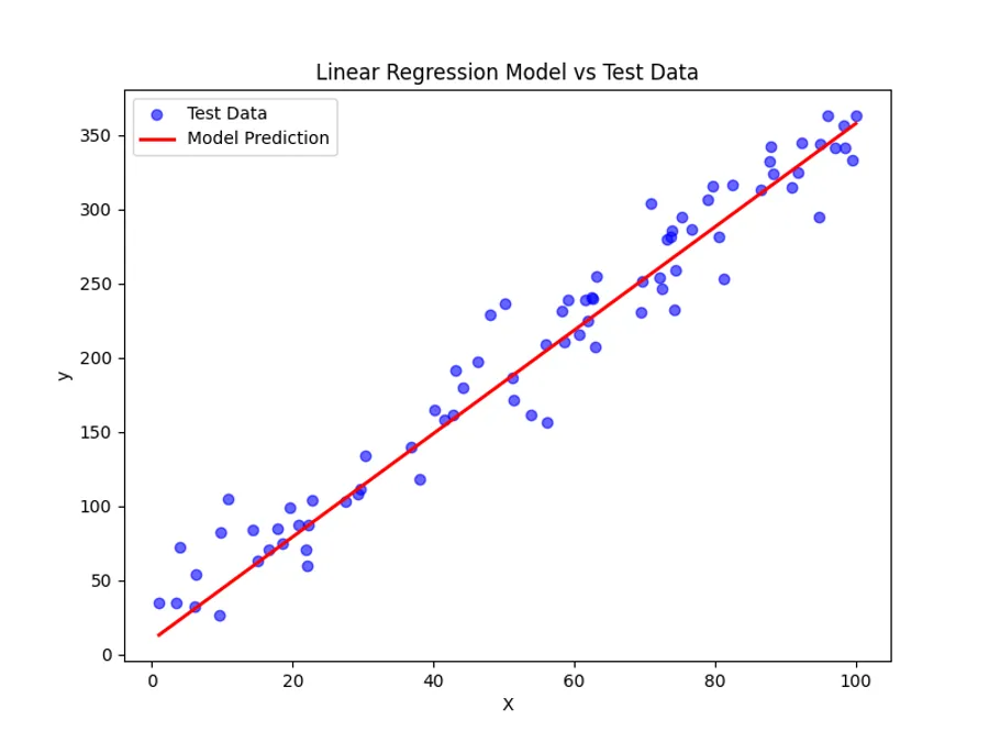
print(f"R² on Test Data = {r2:.2f}") # R² on Test Data = 0.95

This implies that our model explains 95% of the variance in the test data. And when we check our weights, we notice that they are quite similar to the ones used to generate the data:

print(f"\nFinal Model: w_1={w_1:.2f}, w_2={w_2:.2f}")
# Final Model: w_1=3.48, w_2=9.57

Finally, we can visualize our model to see how well it fits the data:

plt.figure(figsize=(8, 6))
plt.scatter(X_test, y_test, color='blue', label='Test Data', alpha=0.6)

x_line = np.linspace(np.min(X_test), np.max(X_test), 100)
y_line = model(x_line, w_1, w_2)
plt.plot(x_line, y_line, color='red', label='Model Prediction', linewidth=2)

plt.xlabel("X")
plt.ylabel("y")
plt.title("Linear Regression Model vs Test Data")
plt.legend()
plt.show()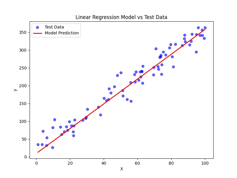

Conclusion

In this post we have seen how to create a simple linear regression model from scratch using Python and NumPy. We have also seen the math behind the model and how to optimize it using the gradient descent algorithm. Hope it helps! :)

Full code can be found in this GitHub