Using Confusion Matrix for Unbalanced Datasets

When working with machine learning models, it’s essential to evaluate the model’s performance accurately. I stumbled upon a new term while learning about model evaluation: confusion matrix. In this post, I’ll showcase that while 0/1 loss gives good accuracy, it’s not always enough information to evaluate the model’s performance.

What is a Confusion Matrix?

Confusion matrix generalizes the basi idea of 0/1 loss, where the classified output differs from the true label. While 0/1 loss gies a single number (what % of the predictions were correct), the confusion matrix gives more detailed view of what the model predictedin multi classification problems.

Let’s consider a small example of a binary classification problem of classifying cats, dogs and rabbits. In this problem, each animal has 100 samples, and the predictions for each class are as follows:

animal	Cat	Dog	Rabbit
Cat	80	15	5
Dog	15	75	10
Rabbit	5	5	90

0/1 loss for cat is 80/100 = 0.8, for dog is 75/100 = 0.75, and for rabbit is 90/100 = 0.9 respectively. But as we can see, creating matrix gives us more information how the distribution between prediction and true label is.

Code Example

Here’s a simple code snippet to generate an imbalanced dataset and analyze its impact using a confusion matrix.

1. Generating an Imbalanced Dataset

First we need to generate some data:

from sklearn.datasets import make_classification
import matplotlib.pyplot as plt
import numpy as np

# 1. Generate an imbalanced dataset
X, y = make_classification(n_classes=2, class_sep=2, 
                           weights=[0.95, 0.05], # 95% dog, 5% cat
                           n_features=5, n_clusters_per_class=1, 
                           n_samples=10000, random_state=42)

# 2. Plot the class distribution
plt.hist(y, bins=np.arange(3)-0.5, edgecolor="black", align="mid")
plt.xticks([0, 1], ["Dog", "Cat"])
plt.title("Class Distribution in the Synthetic Dataset")
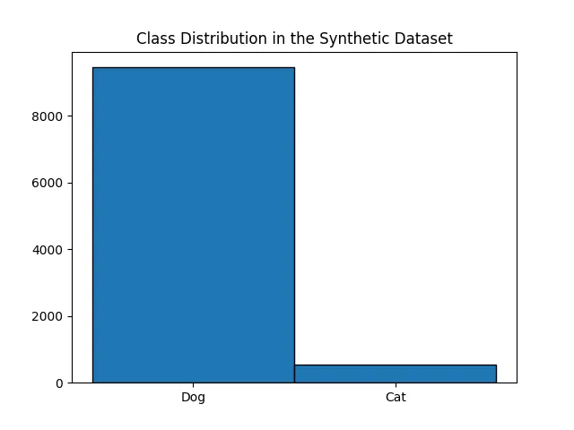
plt.show()

This results in an imbalanced dataset, as shown in the histogram below:

2. Training a Model and Analyzing the Confusion Matrix

Now, let’s train a simple logistic regression model and evaluate its performance.

X_train, X_test, y_train, y_test = train_test_split(X, y, test_size=0.2, random_state=42)

clf = LogisticRegression()
clf.fit(X_train, y_train)
y_pred = clf.predict(X_test)

# Calculate the confusion matrix
accuracy = accuracy_score(y_test, y_pred)
conf_matrix = confusion_matrix(y_test, y_pred)

print(f"Accuracy (0/1 Loss): {accuracy:.2f}")
print("Confusion Matrix:")
print(conf_matrix)

# Visualize the confusion matrix
plt.figure(figsize=(6, 4))
sns.heatmap(conf_matrix, annot=True, fmt="d", cmap="Blues")
plt.xlabel("Predicted Label")
plt.ylabel("True Label")
plt.title("Confusion Matrix")
plt.show()

At first glance, the model seems to perform well with an accuracy of 0.99! But looking at the confusion matrix tells a different story:

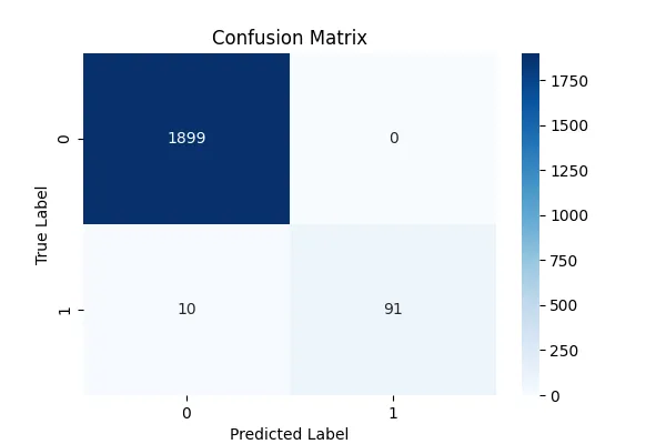
From the matrix, we see that the model correctly predicts almost all majority-class samples (dogs) but struggles significantly with the minority class (cats). This imbalance means that while the accuracy appears high, the model fails to learn useful patterns for the minority class.

Learnings and Takeaways

Using a confusion matrix helps us go beyond simple accuracy and understand where a model struggles. In unbalanced datasets, accuracy alone can be deceptive,, thus other metrics like precision, recall, and F1-score can provide a more comprehensive view of the model’s performance.

For the full code, visit my GitHub repository: Confusion Matrix Evaluation.