Building a Soft Margin SVM in Python with a Quadratic Solver

Support Vector Machine (SVM) is a powerful way to classify binary labeled data. In this post I go over the math behind SVM and how to implement a soft margin SVM in Python using a quadratic solver.

What is Support Vector Machine?

As noted, SVM is a supervised machine learning algorithm for classification tasks. For a binary classification tasks, we have two distinct data classes

\mathcal{C}^{(y=1)} = \{\mathbf{x}^{(i)} : y^{(i)} = 1\}, \quad \text{and} \quad \mathcal{C}^{(y=-1)} = \{\mathbf{x}^{(i)} : y^{(i)} = -1\}.

SVM tries to find a hyperplane that separates the two classes with the maximum margin.

\underbrace{h(\mathbf{x}^{(i)})}_{\mathbf{w}^{\top} \mathbf{x}^{(i)}} > 0 \text{ for } \mathbf{x}^{(i)} \in \mathcal{C}^{(y=1)} \quad \text{and} \quad \underbrace{h(\mathbf{x}^{(i)})}_{\mathbf{w}^{\top} \mathbf{x}^{(i)}} < 0 \text{ for } \mathbf{x}^{(i)} \in \mathcal{C}^{(y=-1)}.

Here’s figure depicting the division of the hyperplane and the data points closest to the hyperplane (also known as support vectors).

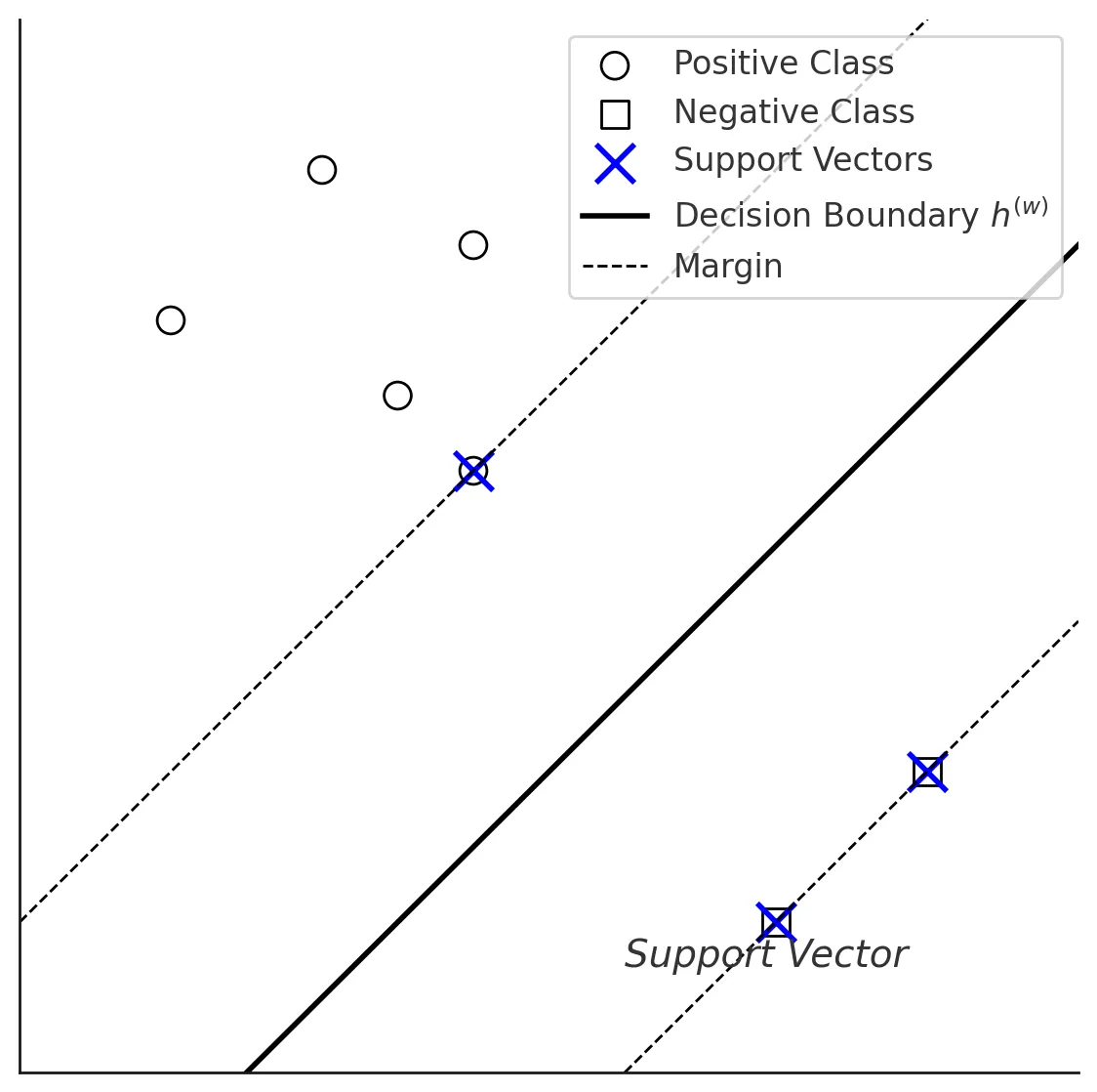
SVM uses the hinge loss function to penalize the misclassification of the data points.

L\bigl((\mathbf{x}, y), h^{(\mathbf{w})}\bigr) := \max\{0, 1 - y \cdot h^{(\mathbf{w})}(\mathbf{x})\} + \lambda \|\mathbf{w}\|_2^2

\underset{h^{(\mathbf{w})}(\mathbf{x}) = \mathbf{w}^{\top} \mathbf{x}}{=} \max\{0, 1 - y \cdot \mathbf{w}^{\top} \mathbf{x}\} + \lambda \|\mathbf{w}\|_2^2.

SVM tries to maximize the distance between the hyperplane and the closest data points. The goal is to find the optimal hyperplane that separates the two classes with the maximum margin.

Larger margin means better generalization to the unseen data. The decision boundary is is defined as:

\mathbf{w}^{\top} \mathbf{x} + b = 0

Which means the line where the boundary changes from one class to another. Because we have binary problem, we know that

Points in the positive class have margin that satisfy $w^T x + b = 1$
Points in the negative class have margin that satisfy $w^T x + b = -1$

The distance from the decision boundary to the data point is thus

\frac{\left| \mathbf{w}^{T} \mathbf{x}_i + b \right|}{\|\mathbf{w}\|}

If point satisfies the margin, then we have

y_i (\mathbf{w}^{T} \mathbf{x}_i + b) \geq 1

Then for support vector machiens we have:

\mathbf{w}^{T} \mathbf{x}_i + b = \pm 1

Which then can be used to calculate the distance from support vector machines to the decision boundary. The distance is then:

\frac{|\pm 1|}{\|\mathbf{w}\|} = \frac{1}{\|\mathbf{w}\|}

Since this is the distance to the decision boundary, our goal is to maximize the overall distance from both sides of the hyperplane. Thus our goal is to get:

\frac{2}{\|\mathbf{w}\|}

This then can be changed into minimization problem:

\min_{\mathbf{w}, b} \|\mathbf{w}\|^2

However, I use

\min_{\mathbf{w}, b} \frac{1}{2} \|\mathbf{w}\|^2

This is because it is easier to take the derivative of the function. This optimization problem is also known as hard margin SVM, due to the fact that it doesn’t allow any misclassification. All data points are correctly classified with margin of at least 1.

y_i (\mathbf{w}^T \mathbf{x}_i + b) \geq 1, \quad \forall i

However, usually the data is not perfectly linearly separable, e.g., there can be outliers that are in the “wrong” side of the decision boundary.

For these cases we can use soft margin SVM, which allows some misclassification.

y_i (\mathbf{w}^T \mathbf{x}_i + b) \geq 1 - \xi_i, \quad \xi_i \geq 0

Thus our optimization problem becomes:

\min_{\mathbf{w}, b, \boldsymbol{\xi}} \quad \frac{1}{2} \|\mathbf{w}\|^2 + C \sum_{i=1}^{n} \xi_i

Where C is a hyperparameter that controls the trade-off between maximizing the margin and minimizing the classification error.

Lagrange Multipliers

To solve the optimization problem, we can use the Lagrange multipliers. Typical optimization problem is of the form:

\min_{\mathbf{w}} \quad f(w)

which is subject to constraints such as

g_i(w) \leq 0 \quad \text{and} \quad h_j(w) = 0.

In SVM setting, we have similar situation, we have optimization problem which is subject to constraints:

y_i (\mathbf{w}^T \mathbf{x}_i + b) \geq 1 - \xi_i, \quad \xi_i \geq 0

We can use the Lagrange multipliers to solve this optimization problem. This means that we introduce new multipliers to our original optimization problem. These are called Lagrange multipliers.

We introduce $a_i \ge 0$ to enforce $y_i (\mathbf{w}^T \mathbf{x}_i + b) \geq 1 - \xi_i$
Similarly, $\mu_i \geq 0$ to enforce $\quad \xi_i \geq 0$

This way we get a new function called Lagrangian function:

\mathcal{L}(\mathbf{w}, b, \boldsymbol{\xi}, \boldsymbol{\alpha}, \boldsymbol{\mu}) = \frac{1}{2} \|\mathbf{w}\|^2 + C \sum_{i=1}^{n} \xi_i - \sum_{i=1}^{n} \alpha_i [ y_i (\mathbf{w}^T \mathbf{x}_i + b) - 1 + \xi_i ] - \sum_{i=1}^{n} \mu_i \xi_i

By introducing these Lagrange multipliers, we can tell the whole objective function in one function. And if the constrains are violated, the Lagrange multipliers will add penalty to the function, thus in order to get optimal solution, Lagrange function needs to find solution that do not violate the constrains!

Deriving the Dual Form

The next step is to derive the dual form of the optimization problem. To do this, we need to find the saddle point of the Lagrangian function. This is done by taking the partial derivatives of the Lagrangian function with respect to the primal variables and setting them to zero.

\frac{\partial \mathcal{L}}{\partial \mathbf{w}} = \mathbf{w} - \sum_{i=1}^{n} \alpha_i y_i \mathbf{x}_i = 0

\mathbf{w} = \sum_{i=1}^{n} \alpha_i y_i \mathbf{x}_i

Then we do it w.r.t. b:

\frac{\partial \mathcal{L}}{\partial b} = - \sum_{i=1}^{n} \alpha_i y_i = 0

finally w.r.t. $\xi_i$ :

\frac{\partial \mathcal{L}}{\partial \xi_i} = C - \alpha_i - \mu_i = 0

Thus we have

$\mathbf{w} = \sum_{i=1}^{n} \alpha_i y_i \mathbf{x}_i$
$\sum_{i=1}^{n} \alpha_i y_i = 0$
$\mu_i = C - \alpha_i$

Substituting these into the Lagrangian function, we get the dual form of the optimization problem:

\max_{\alpha} \sum_{i=1}^{n} \alpha_i - \frac{1}{2} \sum_{i=1}^{n} \sum_{j=1}^{n} \alpha_i \alpha_j y_i y_j (\mathbf{x}_i^T \mathbf{x}_j)

subject to:

\sum_{i=1}^{n} \alpha_i y_i = 0, \quad 0 \leq \alpha_i \leq C

This problem is a quadratic programming problem, which can be solved using standard optimization techniques.

Code Implementation

Now that we have the math behind the SVM, let’s implement it in Python. First we need to import the necessary libraries and generate some data to work with.

import numpy as np
import matplotlib.pyplot as plt
from cvxopt import matrix, solvers

np.random.seed(42)
n_samples = 50

X1 = np.random.randn(n_samples, 2) * 1.0 + np.array([-1, -1])
y1 = -1 * np.ones(n_samples)

X2 = np.random.randn(n_samples, 2) * 1.0 + np.array([1, 1])
y2 = np.ones(n_samples)

X = np.vstack([X1, X2])
y = np.hstack([y1, y2])

Now that we have our data, we can implement the SVM using the quadratic solver.

def svm_solver(X, y, C=1.0):
    N = X.shape[0]

    # Convert y to a column vector
    y = y.astype(float).reshape(-1, 1)

    # Compute the Gram matrix: K[i,j] = X[i] dot X[j]
    K = np.dot(X, X.T)

    # P[i,j] = y_i y_j (X[i] dot X[j])
    P = matrix(np.outer(y, y) * K, tc='d')

    # q is a vector of -1's (because we are minimizing -sum(α))
    q = matrix(-np.ones((N, 1)), tc='d')

    # Inequality constraints: 0 ≤ α_i ≤ C
    G_std = -np.eye(N)  # -α_i ≤ 0  =>  α_i ≥ 0
    G_slack = np.eye(N) # α_i ≤ C
    G = matrix(np.vstack((G_std, G_slack)), tc='d')

    h_std = np.zeros(N)
    h_slack = np.ones(N) * C
    h = matrix(np.hstack((h_std, h_slack)), tc='d')

    # Equality constraint: sum(α_i y_i) = 0
    A = matrix(y.reshape(1, -1), tc='d')
    b = matrix(np.zeros(1), tc='d')

    # Solve QP problem using cvxopt
    solvers.options['show_progress'] = False
    solution = solvers.qp(P, q, G, h, A, b)

    alpha = np.ravel(solution['x'])
    return alpha

Here we have implemented the SVM solver using the quadratic solver from the cvxopt library. Let’s note some things about the code:

Most quadratic solvers require the optimization problem to be in the form of:

\min_{x} \frac{1}{2} x^T P x + q^T x

Thus we negated our objective function to make it a minimization problem.

\min_{\alpha} \frac{1}{2} \sum_{i,j} \alpha_i \alpha_j y_i y_j \left( x_i^T x_j \right) - \sum_{i=1}^{n} \alpha_i

Then in the code I introduced P and q:

P is the matrix of the form $y_i y_j (x_i^T x_j)$
q is the vector of -1’s

The constrains are same as before.

After solving the alpha values, we can calculate the weights and the bias:

alpha = svm_solver(X, y, C=C)

def compute_w_b(alpha, X, y, C=1.0, threshold=1e-5):
    w = np.sum((alpha * y.reshape(-1))[:, None] * X, axis=0)
    support_indices = np.where((alpha > threshold) & (alpha < C - threshold))[0]
    if len(support_indices) == 0:
        support_indices = np.where(alpha > threshold)[0]
    b_values = [y[i] - np.dot(w, X[i]) for i in support_indices]
    b = np.mean(b_values)
    return w, b, support_indices
w, b, support_indices = compute_w_b(alpha, X, y, C=C)
print("Weight vector w:", w)
print("Bias b:", b)

Weight vector w: [1.29003989 1.28460522] Bias b: -0.028575582255710146

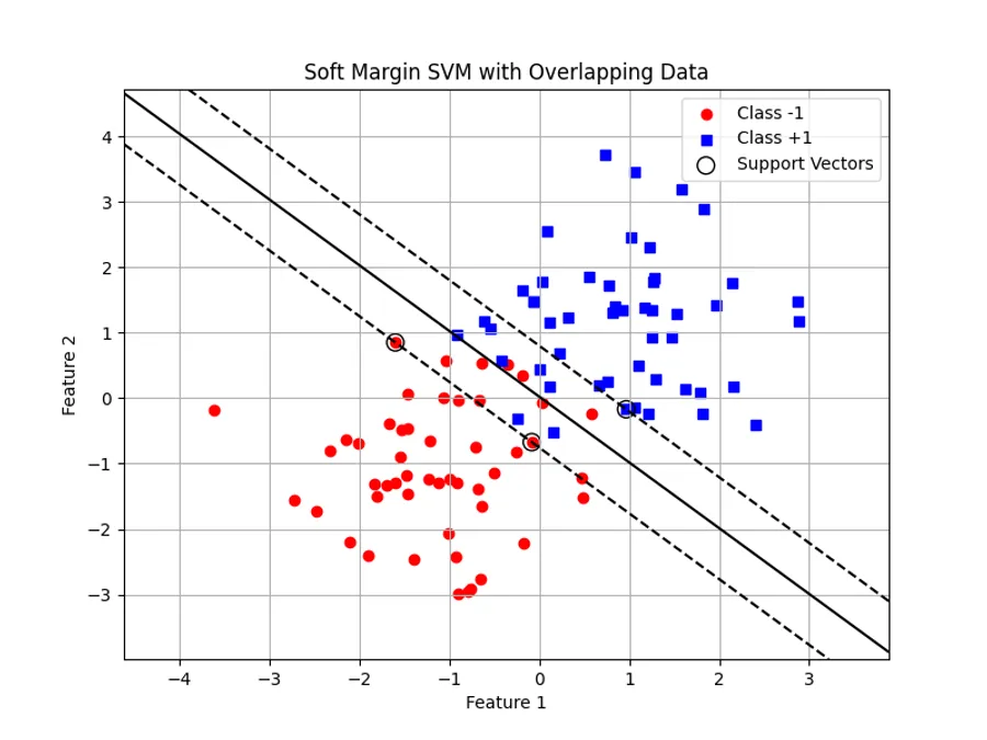
Finally, we can plot the decision boundary

Conclusion

In this post, we have implemented the soft margin SVM solver using the quadratic solver from the cvxopt library. We have also shown how to compute the weight vector and the bias term. Finally, we have plotted the decision boundary.

As usual, the code is available on my GitHub

Thank you for reading! :)