Building Coordinate Descent for Lasso Loss from Scratch

Many times when working with data in machine learning, we do not know before hand which features are the most important. This is especially true in situations where we have a large number of features. In this post I go over Lasso loss, which is a loss function that can be used to perform feature selection, and how to optimize the weights of the Lasso loss using coordinate descent.

What is Lasso loss

Before going over the function for Lasso loss, let’s first go over the mean squared error (MSE):

MSE = \frac{1}{N} \sum_{i=1}^{N} (y_i - \hat{y}_i)^2

The Lasso loss is a regularized version of the MSE. It adds a penalty term to the MSE, which penalizes the model if it tries to use too many features.

Lasso = \frac{1}{N} \sum_{i=1}^{N} (y_i - \hat{y}_i)^2 + \lambda \sum_{j=1}^{M} |w_j|

Where $\lambda$ is a hyperparameter that controls how much we want to penalize the model for using too many features.

Coordinate Descent for Lasso Loss

Our goal here is the same as in the polynomial or linear regression case: we want to find the weights that minimize the Lasso loss. However, we notice that we can’t use the gradient descent algorithm because the penalizing term is not differentiable at 0!

So instead of going over all the weights at the same time, we can optimize one weight at a time while keeping the others fixed. This is called coordinate descent.

The basic idea goes like this:

Initialize the weights to 0.
For each weight, find the value that minimizes the Lasso loss while keeping the other weights fixed. This is a one-dimensional optimization problem, which can be solved using a simple line search.
Repeat step 2 until convergence.

So let’s calculate how to update the weights for linear regression!

Coordinate Descent for Linear Regression

Here’s basic model for linear regression:

\|\,y - Xw\,\|_{2}^{2} \;=\; \sum_{i=1}^{N} \bigl(y_{i} - (x_{i} \cdot w)\bigr)^{2}.

Thus when we plug it to our Lasso loss, we get:

\mathcal{L}(w) \;=\; \underbrace{\frac{1}{2N}\,\|y - X\,w\|_{2}^{2}}_{\text{MSE part}} \;+\;\alpha\,\|w\|_{1}

Here we used small trick to make the derivative of the MSE part easier to compute. We divided the MSE part by 1/2, because $\frac{ \delta }{ \delta w } (y-Xw)^{2} =2(y-Xw)X$ , thus dividing it by 2 we get $\frac{ \delta }{ \delta w } (y-Xw)^{2} = (y-Xw)X$ , which is simpler to work with.

Coordinate Setup

We need to optimize this loss function one weight at a time, by putting all other weights to be constant.

For a given weight $w_{j}$ , we can define the estimate as:

\hat{y}_i = X_{ij}\,w_j \;+\; \sum_{k \neq j} X_{ik}\,w_k.

Thus the error for the $i$ -th sample is:

e_i = y_i - \hat{y}_i

But from this we notice, that the $y_i - \sum_{k \neq j} X_{ik}\,w_k$ is constant for a given $w_j$ , so we can define:

r_i = y_i - \sum_{k \neq j} X_{ik}\,w_k

This is called as residual, and it is the part of the target that is not explained by the other weights. Using residual in our error equation we get:

e_i = y_i - \hat{y}_i = r_i - X_{ij}\,w_j

Finally we can use this in our loss function, where goal is to minimize the error.

\min_{w_j} \;\frac{1}{2N}\sum_{i=1}^N \bigl(r_i - X_{ij}\,w_j\bigr)^{2} \;+\;\alpha\,\lvert w_j\rvert

We can differentiate the quadratic part of the function. Let’s define it as $Q = \frac{1}{2N}\sum_{i=1}^N \bigl(r_i - X_{ij}\,w_j\bigr)^{2}$

\frac{dQ}{dw_j} = \frac{1}{2N} \sum_{i=1}^N \bigl(-2\,r_i\,X_{ij} \;+\; 2\,X_{ij}^2\,w_j \bigr) = \frac{1}{N}\,\Bigl(\sum_{i=1}^N X_{ij}^2\,w_j \;-\; \sum_{i=1}^N r_i\,X_{ij}\Bigr).

From here we can define two variables (to ease computations):

z_j = \sum_{i=1}^{N} X_{ij}^2,

\tilde{\rho}_j = \sum_{i=1}^{N} X_{ij}\,r_i.

So our function becomes

\frac{dQ}{dw_j} = \frac{1}{N}\bigl(z_j\,w_j - \tilde{\rho}_j\bigr).

Handling the Lasso Penalty Term

However, as we know, there is also the lasso penalty term that needs to be taken care of in the lasso loss. As the $\alpha \,\lvert w_j\rvert.$ is the penalty term, it’s derivate is not defined in $w_{j} = 0$ !

However, we can use the subgradient of the absolute value function, which is defined as:

\frac{d}{dw_j}\lvert w_j\rvert = \begin{cases} \mathrm{sign}(w_j) & \text{if } w_j \neq 0,\\[6pt] \text{any value in }[-1, 1] & \text{if } w_j = 0. \end{cases}

Thus the whole subgradient function $f(w_{j})$ becomes:

f'(w_j) = \frac{1}{N}\bigl(z_j\,w_j - \tilde{\rho}_j\bigr) \;+\;\alpha\,\mathrm{sign}(w_j)

Now we can try to find the optimal by setting subgradient to zero:

\frac{1}{N}\bigl(z_j\,w_j - \tilde{\rho}_j\bigr) \;+\;\alpha\,\mathrm{sign}(w_j) \;=\; 0.

and from this we can get the optimal w!

w_j = \frac{\tilde{\rho}_j \;-\; \alpha\,N\,\mathrm{sign}(w_j)}{z_j}

Soft-Thresholding Function

We already have our optimal $w_j$ , but we must take care of the sign function.

Let’s first notice how the function behaves for different values.

$w_{j} > 0; sign(w_{j}) = 1$ , thus the update is

w_j = \frac{\tilde{\rho}_j \;-\; \alpha\,N}{z_j}

An in order to make sure that $w_{j} > 0$ we need to have $\tilde{\rho}_{j} > \alpha N$ .

$w_{j} < 0; sign(w_{j}) = -1$ , thus the update is

w_j = \frac{\tilde{\rho}_j \;+\; \alpha\,N}{z_j}

For this to be negative we need to have $\tilde{\rho}_{j} < -\alpha N$ .

$\lvert \tilde{\rho}_j\rvert \;\le\; \alpha\,N.$

OK, so from the positive and negative cases, we know when they hold. But there is also the case $-\alpha N \;\le\; \tilde{\rho}_j \;\le\; \alpha N.$ In that zone, neither the positive and negative case holds, and giving value to $w_{j}$ contradicts the arguments! So only viable option is to set $w_{j} = 0$ .

Putting all these together we get:

w_j = \begin{cases} \dfrac{\tilde{\rho}_j - \alpha\,N}{z_j}, & \tilde{\rho}_j > \alpha\,N,\\[6pt] 0, & \lvert \tilde{\rho}_j\rvert \;\le\; \alpha\,N,\\[6pt] \dfrac{\tilde{\rho}_j + \alpha\,N}{z_j}, & \tilde{\rho}_j < -\alpha\,N. \end{cases}

From this we can define soft-thresholding function $S(a,\lambda)$

S(a,\lambda) = \begin{cases} a - \lambda, & a > \lambda,\\[6pt] 0, & \lvert a\rvert \le \lambda,\\[6pt] a + \lambda, & a < -\lambda. \end{cases}

Where $\lambda \;\leftrightarrow\; \alpha\,N.$ and $a\;\leftrightarrow\; \tilde{\rho}_j,$ This can also be put to single-formula version: $S(a,\lambda) = \text{sign}(a) \cdot \max(\lvert a\rvert - \lambda, 0).$

Thus our final function becomes:

w_j = \frac{S\bigl(\tilde{\rho}_j, \alpha\,N\bigr)}{z_j}

Using soft-thresholding function in Python

Now that we know the math behind the coordinate descent, we can start implementing it in Python!

Let’s again start by generating data and initializing the variables:

import numpy as np
np.random.seed(42)

n_samples, n_features = 200, 10
X = np.random.randn(n_samples, n_features)

true_w = np.zeros(n_features)
true_w[0] = 2.0
true_w[3] = -1.5
true_w[7] = 3.0

y = X @ true_w + 0.5 * np.random.randn(n_samples)
N = len(y)

Then we define the training and test set from this data

train_ratio = 0.8 # Train-Test Split Ratio
train_size = int(N * train_ratio)

indices = np.random.permutation(N)
train_idx, test_idx = indices[:train_size], indices[train_size:]

X_train, y_train = X[train_idx], y[train_idx]
X_test, y_test = X[test_idx], y[test_idx]

In this example, I use linear regression and MSE, like in the math section of this post. I also define here the soft-thresholding function which is the key part of the coordinate descent algorithm.

def model(X, weights):
    return X @ weights

def mse(y_true, y_pred):
    return np.mean((y_true - y_pred)**2)

def soft_thresholding(x, alpha):
    return np.sign(x)* np.maximum(np.abs(x) - alpha, 0)

Finally we can define our coordinate descent function:

def coordinate_descent_lasso(X, y, alpha = 0.1, max_iter = 10000, tol = 1e-6):
    w = np.zeros(n_features)

    for _ in range(max_iter):
        w_old = w.copy()

        for j in range(n_features):
            
            residual = y - X.dot(w)
            rho_j = X[:, j].dot(residual)
            z_j =  np.sum(X[:, j]**2)
            w[j] = soft_thresholding(rho_j, alpha * train_size) / z_j


        if np.linalg.norm(w - w_old) < tol:
                break
    
    return w

w_estimated = coordinate_descent_lasso(X_train, y_train, alpha = 0.1, max_iter = 10000, tol = 1e-6)
print("Estimated weights:",w_estimated)

Let’s stop here for a moment to analyze the code.

The algorithm itself is quite similar to the gradient descent, we both have iteration over the data and we update the weights. However, in this case, we do the update one feature at a time.

$r_{i}$ , $\rho_{j}$ and $z_{j}$ are defined as same as in the math section. And the update rule is the soft-thresholding function, is also the same:

w_j = \frac{S\bigl(\tilde{\rho}_j, \alpha\,N\bigr)}{z_j}

Model Evaluation

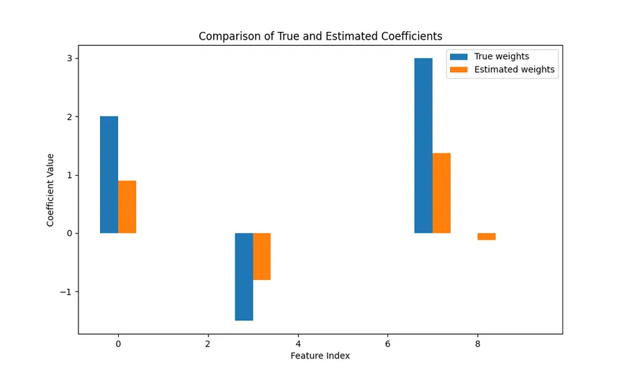
Finally, we can check the results of our model, and see if it does the feature selection correctly.

Parameter	Value
Estimated weights	`[ 0.90319841, -0, -0, -0.8026248, 0, 0, 0, 1.36803295, -0.12094796, -0 ]`
Test MSE	`4.376614616021284`
Test R² Score	`0.6883895004659537`

As we can see, the model actually put most of the irrelevant features to zero. Also the relevant features have similar behaviour in weights as in the true model.

But we notice that the weights are actually smaller than the one in the true model.

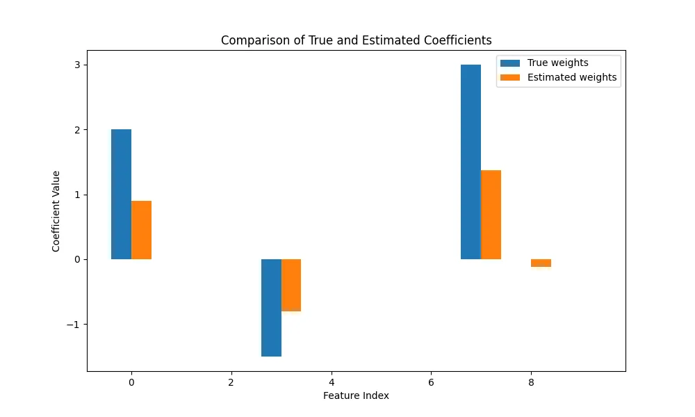
This is common charactericstic of Lasso regression, as Lasso adds penalty to the loss function, it also forces the the estimated coefficient closer to zero. This means that coefficient tend to be smaller in absolute value than the true coefficient.

However, given that MSE and R² score are reasonable, this result is generally good from predictive standpoint. It shows that even though the coefficients are biased, the model overall captures the relationship in the data well.

Summary

In this post I went through the math behind the Lasso loss and how it can be calculated using Coordinate descent. After that I implemented the Lasso regression from Scratch using python, which helped us to select the relevant features from the data.

For the full code, check out the Github repository. Thanks for reading! :)